Thread by Ben Collins
- Tweet
- Jul 19, 2022
- #ComputerScience #CareerDevelopment
Thread
Today's #GoogleSheets tip wasn't ever meant to be a tip. I was just trying to scrape some data for another tip...
But creating the formula was so interesting (and, dare I say, fun! 😜) that I decided to share it instead.
Buckle up... We're in for a wild ride!
But creating the formula was so interesting (and, dare I say, fun! 😜) that I decided to share it instead.
Buckle up... We're in for a wild ride!
Here's the problem we're going to solve with today's tip ⬇️
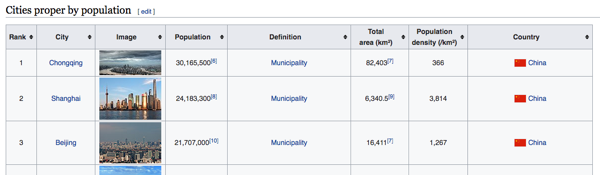
We want to scrape the population data from this table in Wikipedia...
We want to scrape the population data from this table in Wikipedia...
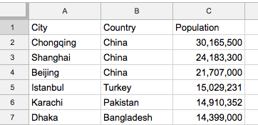
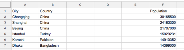
... and put it into a Google Sheet like this, so we can use it for analysis.
The challenge today is to do this with a single formula!
Ready? Let's jump in!
The challenge today is to do this with a single formula!
Ready? Let's jump in!
1️⃣ Open a new Google Sheet.
2️⃣ In cell A1, insert a basic IMPORTHTML formula to scrape the raw table of population data from Wikipedia:
=IMPORTHTML("en.wikipedia.org/wiki/List_of_cities_proper_by_population","table",2)
The data has some issues, but it's a start.
2️⃣ In cell A1, insert a basic IMPORTHTML formula to scrape the raw table of population data from Wikipedia:
=IMPORTHTML("en.wikipedia.org/wiki/List_of_cities_proper_by_population","table",2)
The data has some issues, but it's a start.

3️⃣ Pick the columns we want, by wrapping the Import formula with a Query formula.
(Use Col1 notation in our Select statement, not the column letter.)
=QUERY(IMPORTHTML("en.wikipedia.org/wiki/List_of_cities_proper_by_population","table",2),"select Col2, Col8, Col4",1)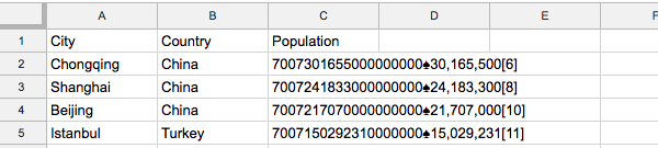
(Use Col1 notation in our Select statement, not the column letter.)
=QUERY(IMPORTHTML("en.wikipedia.org/wiki/List_of_cities_proper_by_population","table",2),"select Col2, Col8, Col4",1)

4️⃣ Hmm, that population column is messed up! Regex to the rescue! ⛑️
At this point, we'll deal with the population column on its own and come back to our main formula later...
At this point, we'll deal with the population column on its own and come back to our main formula later...
So make a copy of this Import formula in cell F1 and change it to:
=QUERY(IMPORTHTML("en.wikipedia.org/wiki/List_of_cities_proper_by_population","table",2),"select Col4",1)
Now we should have a copy of just the population column in column F.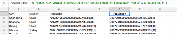
=QUERY(IMPORTHTML("en.wikipedia.org/wiki/List_of_cities_proper_by_population","table",2),"select Col4",1)
Now we should have a copy of just the population column in column F.

5️⃣ Wrap this population only formula in cell F1 with a Regex formula:
=REGEXEXTRACT(QUERY(IMPORTHTML("en.wikipedia.org/wiki/List_of_cities_proper_by_population","table",2),"select Col4",1),"♠([0-9,]*)")
Hmm, that gives us a #N/A error... 🤔
=REGEXEXTRACT(QUERY(IMPORTHTML("en.wikipedia.org/wiki/List_of_cities_proper_by_population","table",2),"select Col4",1),"♠([0-9,]*)")
Hmm, that gives us a #N/A error... 🤔
6️⃣ Turn this into an Array Formula and get the column of population numbers!
=ARRAYFORMULA(REGEXEXTRACT(QUERY(IMPORTHTML("en.wikipedia.org/wiki/List_of_cities_proper_by_population","table",2),"select Col4",1),"♠([0-9,]*)"))
=ARRAYFORMULA(REGEXEXTRACT(QUERY(IMPORTHTML("en.wikipedia.org/wiki/List_of_cities_proper_by_population","table",2),"select Col4",1),"♠([0-9,]*)"))

The Regex formula uses this expression "♠([0-9,]*)" to extract the numbers after the funny ♠ symbol.
We still have two problems to solve though:
🔹 we need to convert the strings into actual numbers and
🔹 fix the #N/A column heading
...
We still have two problems to solve though:
🔹 we need to convert the strings into actual numbers and
🔹 fix the #N/A column heading
...
7️⃣ Use the SUBSTITUTE function to remove the commas and convert the strings into numbers:
=ARRAYFORMULA(SUBSTITUTE(REGEXEXTRACT(QUERY(IMPORTHTML("en.wikipedia.org/wiki/List_of_cities_proper_by_population","table",2),"select Col4",1),"♠([0-9,]*)"),",","")*1)
=ARRAYFORMULA(SUBSTITUTE(REGEXEXTRACT(QUERY(IMPORTHTML("en.wikipedia.org/wiki/List_of_cities_proper_by_population","table",2),"select Col4",1),"♠([0-9,]*)"),",","")*1)
(The multiplication by 1 at the very end coerces the strings into numbers after the commas have been removed.)
8️⃣ Use the IFERROR function to fix that pesky #N/A error at the top of our column heading, and replace the #N/A with the word "Population"...
=ARRAYFORMULA(IFERROR(SUBSTITUTE(REGEXEXTRACT(QUERY(IMPORTHTML("en.wikipedia.org/wiki/List_of_cities_proper_by_population","table",2),"select Col4",1),"♠([0-9,]*)"),",","")*1,"Population"))
Nice, now we have our population column as numbers.
Nice, now we have our population column as numbers.

9️⃣ Go back to the main formula in A1 and remove the old population column (with the funny numbers). Our formula in A1 should now be:
=QUERY(IMPORTHTML("en.wikipedia.org/wiki/List_of_cities_proper_by_population","table",2),"select Col2, Col8",1)
=QUERY(IMPORTHTML("en.wikipedia.org/wiki/List_of_cities_proper_by_population","table",2),"select Col2, Col8",1)
🔟 All that's left is to join these two ranges, in columns A, B and F, using the curly bracket notation.
This formula is too big to fit in one tweet, so I'm going to have to split it. Forgive me!
={
QUERY(IMPORTHTML("en.wikipedia.org/wiki/List_of_cities_proper_by_population", "table",2),"select Col2, Col8",1)
,
This formula is too big to fit in one tweet, so I'm going to have to split it. Forgive me!
={
QUERY(IMPORTHTML("en.wikipedia.org/wiki/List_of_cities_proper_by_population", "table",2),"select Col2, Col8",1)
,
ARRAYFORMULA(IFERROR(SUBSTITUTE(REGEXEXTRACT(QUERY(IMPORTHTML("en.wikipedia.org/wiki/List_of_cities_proper_by_population","table",2),"select Col4",1),"♠([0-9,]*)"),",","")*1,"Population"))
}
We're done! 🤪 Here's the output.
(You can delete the workings in column F.)
}
We're done! 🤪 Here's the output.
(You can delete the workings in column F.)

Yes, it would have been quicker to cut and paste the table from Wikipedia and fix the funny formats manually.
But where's the fun in that? 🤣
Think of this as an exercise in combining some of the most useful single functions in Google Sheets to create really powerful formulas.
But where's the fun in that? 🤣
Think of this as an exercise in combining some of the most useful single functions in Google Sheets to create really powerful formulas.
By the way, my free 30 Day Advanced Formulas course covers all of the functions/formulas we used today...
🔹 Query function: days 14 and 15
🔹 Array formulas: day 17
🔹 Import function: day 19
🔹 Regex function: day 20
You can take the course for free at courses.benlcollins.com/p/advanced30/
🔹 Query function: days 14 and 15
🔹 Array formulas: day 17
🔹 Import function: day 19
🔹 Regex function: day 20
You can take the course for free at courses.benlcollins.com/p/advanced30/